Workshop Guide

Hello re:Invent workshoppers! We are excited for you to join us to learn how to build and monitor a serverless application!

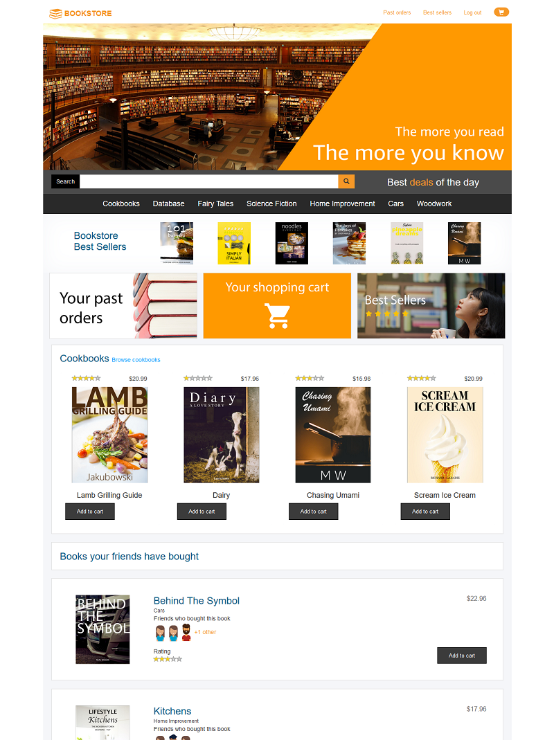
The AWS Bookstore Demo App is a full-stack sample web application that creates a storefront (and backend) for customers to shop for fictitious books. You can browse and search for books, look at recommendations and best sellers, manage your cart, check out, view your orders, and more.

The bookstore demo app screen shot

The goal of the AWS Bookstore Demo App is to provide a fully-functional web application that uses multiple, purpose-built AWS databases and native AWS components like Amazon API Gateway and AWS CodePipeline. Increasingly, modern web apps are built using a multitude of different databases. Developers break their large applications into individual components and select the best database for each job. Let's consider the AWS Bookstore Demo App as an example. The app contains multiple experiences such a shopping cart, product search, recommendations, and a top sellers list. For each of these use cases, the app makes use of a purpose-built database so the developer never has to compromise on functionality, performance, or scale.

The Bookstore Demo App is a stand-alone application. You can deploy and learn from it as-is. Part of building any application is ensuring that it performs well, that the infrastructure is serving traffic in a timely way, finding and removing bugs, and maintaining a secure environment. In this lab, you will extend the Bookstore Demo App, adding AWS X-Ray tracing for its underlying functions. You will flow X-Ray (trace), and application data to Amazon Elasticsearch Service (Amazon ES). You will use Amazon ES to build dashboards to monitor the Bookstore Demo App in real time.

If you complete this workshop in its entirety, good for you! We are very impressed. This workshop is not only designed to help you learn how to leverage these application templates, but also it is intended to leave you with ideas for how you might change and extend these (or other) applications in the future.

There are several advanced sections to the workshop (marked as optional) that you can take home with you after the workshop session.

We are excited for you to join us to learn how to build your own stack in just a few clicks!

The Bookstore

Play with the deployed Bookstore

AWS Bookstore Demo App is a full-stack sample web application that creates a storefront (and backend) for customers to shop for fictitious books. You can browse and search for books, look at recommendations and best sellers, manage your cart, checkout, view your orders, and more.

Try out the deployed application here! This will open a new window with a fully-deployed version of AWS Bookstore Demo App. Sign up using an email address and password (choose Sign up to explore the demo). Note: Given that this is a demo application, we highly suggest that you do not use an email and password combination that you use for other purposes (such as an AWS account, email, or e-commerce site).

Once you provide your credentials, you will receive a verification code at the email address you provided. Upon entering this verification code, you will be signed into the application.

View the different product categories, add some items to your cart, and checkout. Search for a few books by title, author, or category using the search bar. View the Best Sellers list, and see if you can move something to the top of the list by ordering a bunch of books. Finally, take a look at the social recommendations on the home page and the Best Sellers page. Look at you, savvy book shopper!

Deploy the AWS Bookstore Demo App

You have received an IAM account to deploy the application. Please use this account to deploy only the CloudFormation template and work with the instructions in this guide. These accounts and their resources will be removed at the end of this event.

If you prefer, you can follow the steps in this guide and create all of the resources in your own AWS account. IMPORTANT NOTE: Creating this application in your AWS account will create and consume AWS resources, which will cost money. We estimate that running this demo application will cost <$0.60/hour with light usage. Be sure to shut down/remove all resources once you are finished with the workshop to avoid ongoing charges to your AWS account (see instructions on cleaning up/tear down in clean up section below.

To get the AWS Bookstore Demo App up and running, follow these steps:

Navigate to the AWS console
- If you are logging in to your own account, log in normally Note:If you are logged in as an IAM user, ensure your account has permissions to create and manage the necessary resources and components for this application.
- If you are using a provided account, use the account Id, user name, and password provided to you to log in as an IAM user.
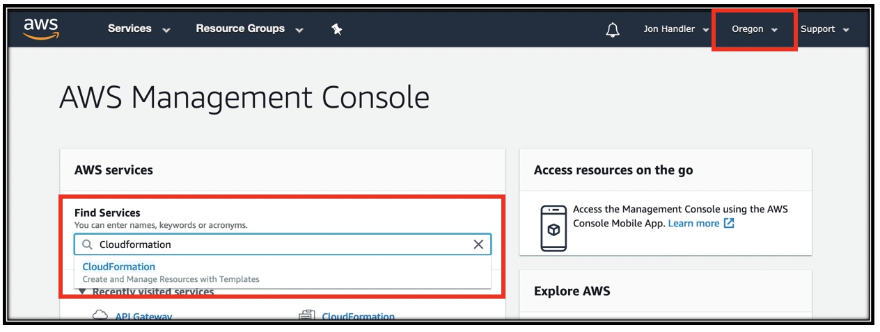
Ensure your region selector is set to US West (Oregon) region
From the main console, enter CloudFormation in the service search box and click CloudFormation in the drop down.
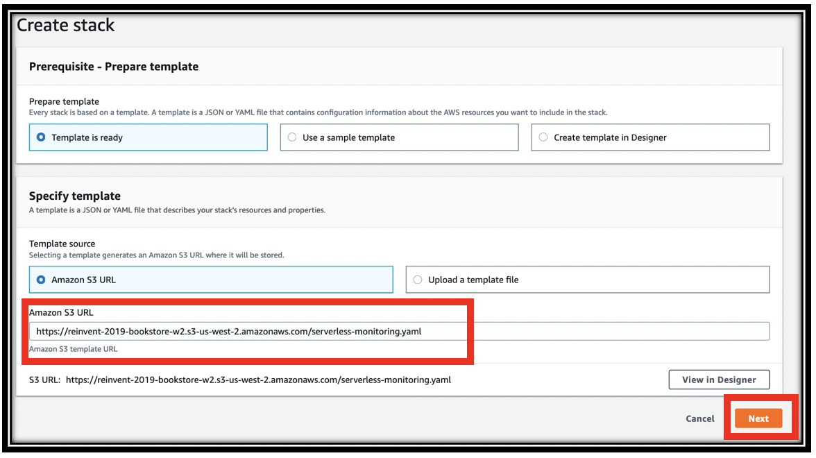
Click Create Stack
Copy the following URL and paste it into the Amazon S3 URL text box. https://aws-bookstore-monitoring-demo.s3.amazonaws.com/serverless-monitoring.yaml
Click Next
Continue through the CloudFormation wizard steps
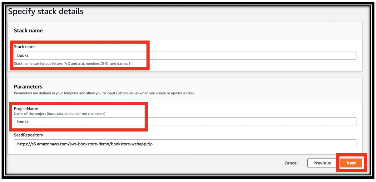
1. Name your stack, e.g. books
2. Provide a project name (must be lowercase, letters only, and under ten characters). This is used when naming your resources, e.g. tables, search domain, etc.
Click Next
In the Configure stack options page, scroll to the bottom and click Next
In the Review page, scroll to the bottom, click the check box next to I acknowledge that AWS CloudFormation might create IAM resources with custom names., then click Create stack. This will take ~20 minutes to complete.

This lab guide will refer back to the CloudFormation template frequently. Download it now and open it with your favorite editor. To download the template, simply copy the URL https://aws-bookstore-monitoring-demo.s3.amazonaws.com/serverless-monitoring.yaml and paste it in your browser's navigation bar.

High level architecture

While the application is deploying in CloudFormation (should take ~20 minutes), let's talk about the architecture. The Bookstore Demo App is built on the AWS full stack template. Both of those links have excellent README.md files that go into depth on the architecture. We recommend that you read them, especially the Bookstore Demo App's README

For this lab, we have added significantly to the Bookstore Demo App to enable monitoring and logging.

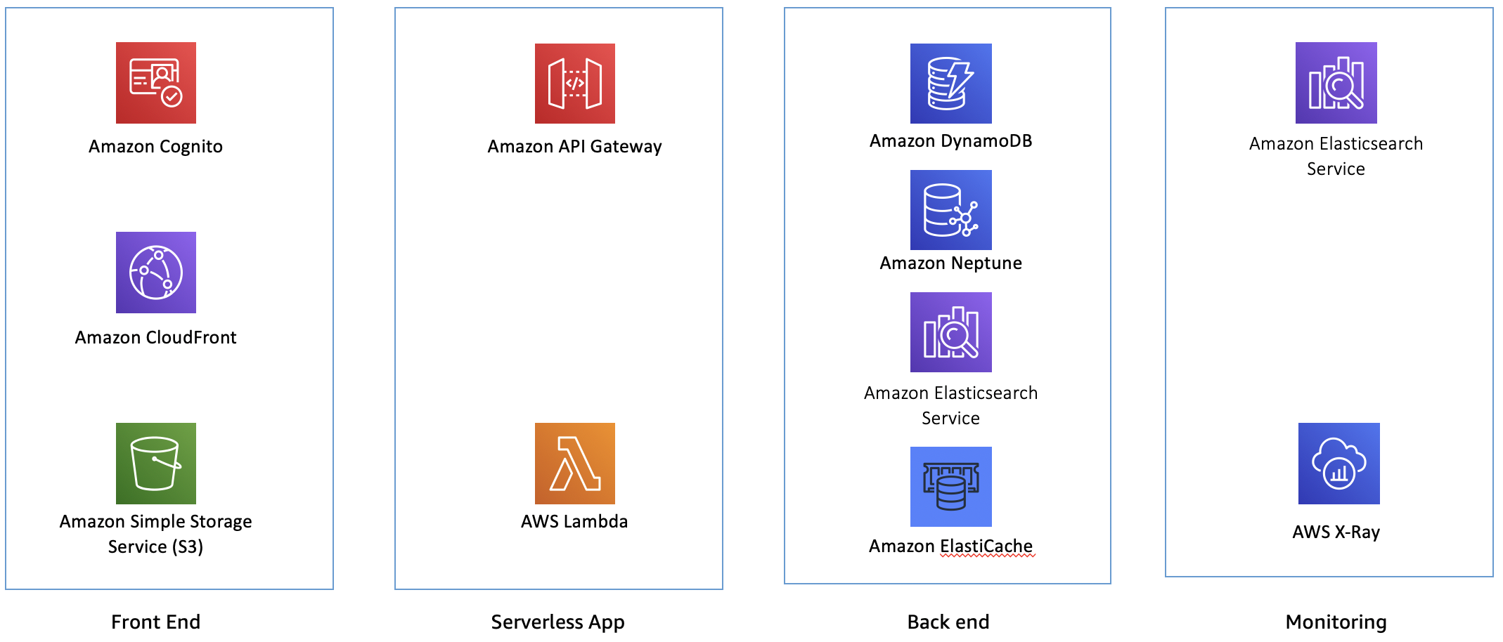
the Bookstore Demo App high level architecture

For the front end, you have Amazon Cognito providing authentication, Amazon CloudFront for serving assets, and Amazon S3 for hosting the application.

In the serverless app layer, you have Amazon API Gateway, backed by AWS Lambda for responding to API requests. All of the application traffic goes through this layer.

In the back end, you have Amazon DynamoDB serving the catalog of books, Amazon Neptune for tracking friends and making recommendations, Amazon Elasticsearch Service providing search across the books catalog, and Amazon Elasticache for Redis for maintaining best seller information.

At the monitoring layer, you have AWS X-Ray for distributed tracing and metrics, and Amazon Elasticsearch service for storing application and X-Ray logs.

Peeling back the onion to the next layer:

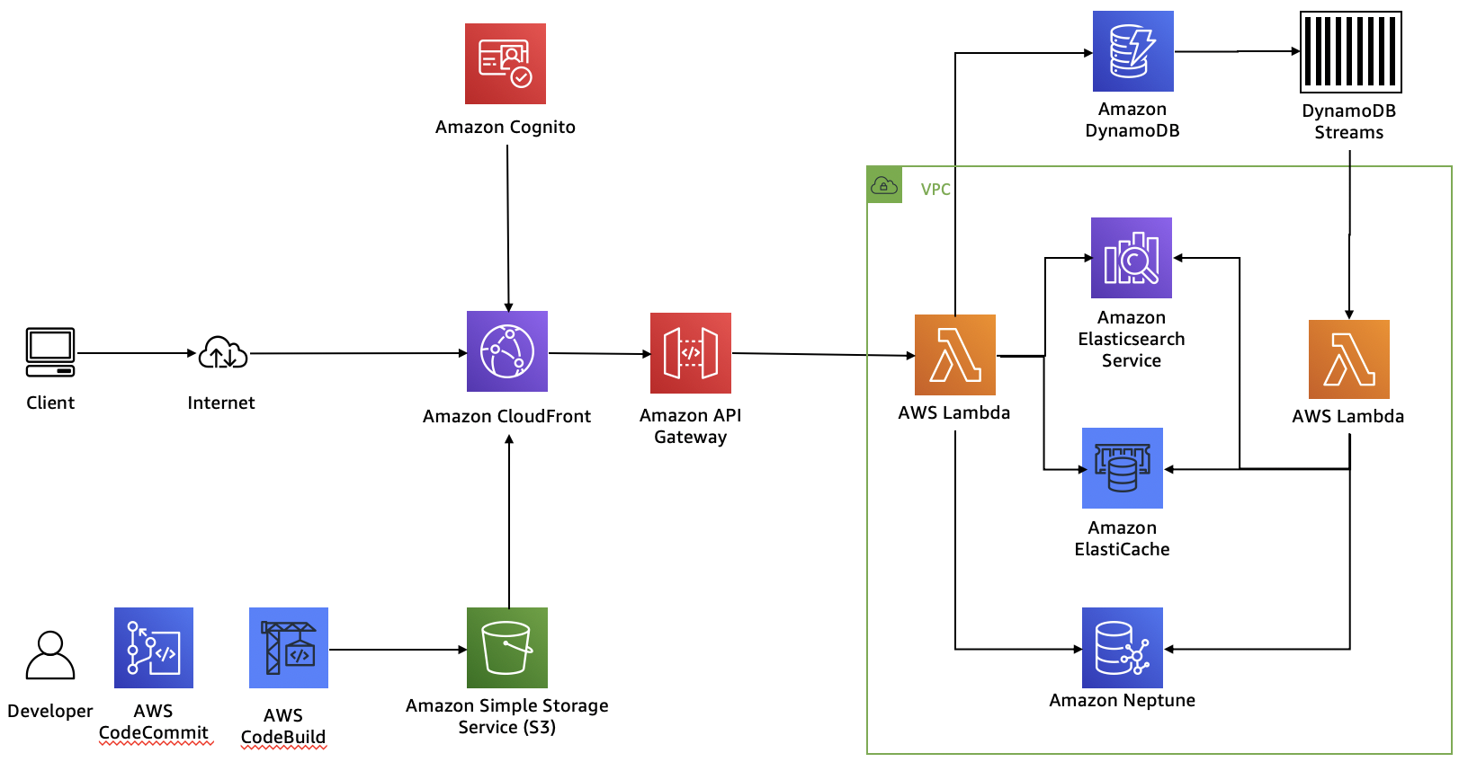
The Bookstore Demo App's application architecture

One pattern for building serverless applications is to use AWS Code Commit and AWS Code Build to create the application artifacts in S3. Amazon CloudFront loads these components and uses them to serve client requests. Along the way, Amazon Cognito provides authentication for website customers.

Amazon API Gateway powers the interface layer between the frontend and backend and invokes Lambda functions that interact with our purpose-built databases.

As updates come into DynamoDB (the database of record), they are sent through DynamoDB streams and an AWS Lambda function to forward changes to the Amazon ES domain, to Elasticache for Redis, and to Neptune.

For the monitoring layer

The Bookstore Demo app monitoring layer

Lambda, API Gateway, and DynamoDB forward information to AWS X-Ray. In this lab, you will use the X-Ray console to explore this information.

We have also added a second Amazon ES domain to hold log data. As a general rule, it's good to separate concerns and host search data in one domain and log data in a different domain. Because these two data types have such different access patterns, they scale quite differently. Also, by placing log data and search data in different domains, you reduce the blast radius. After all, you don't want a problem with your logs preventing search on your front end application.

We chose to deploy the second Amazon ES domain outside of the VPC. This is really an anti-pattern. Best practice is to keep logging information inside the VPC, along with other sensitive data. We did it this way because providing access to the Amazon ES endpoint inside the VPC would greatly complicate the labs architecture, template, and this guide. This is a simplification that we chose because the data is not critical.

There are two sources of log data – AWS X-Ray and inline logging code in the Search, addToCart, and Checkout Lambda functions. We instrumented each of these Lambda functions, and we encourage you to have a look at them once they're deployed (we'll refer to this code throughout the lab guide).

To get X-Ray data, we built a scheduled Lambda that runs every minute, pulling data from X-Ray and sending it to Amazon ES.

In all cases, we used an Amazon Simple Queue Service (SQS) queue to collect data. We use a triggered Lambda to collect data from the queue and forward it to Amazon ES. This pattern is a very common part of any logging solution. While each component can send messages directly to Amazon ES, you will eventually overwhelm Amazon ES with too much concurrency. SQS serves here as a buffering layer to reduce concurrent connections.

If your stack has not finished deploying, browse the readme for AWS Bookstore Demo App. The Overview section provides a basic understanding of what the application consists of. The remainder of the readme file dives deeper, including the Architecture, Implementation details, and Considerations for demo purposes sections. This familiarization with how the app is structured will come in handy once deployment is complete and we browse the components of the application.

Dive into the back end

Now that the application is up and running, let's open the hood and play around with some of the backend componentry.

Go back to the CloudFormation console, open the stack details page for your application, go to the Outputs table, and find the WebApplication URL. This is the public endpoint to your deployed application. Click the link to open and explore your brand-new Bookstore!

Since this is a completely new instance of the application, your username and password that you used before in Step 1 won't work. Sign up for an account in your Bookstore, and test out the app! Test to make sure the email verification works, and run through some of use cases like search, cart, ordering, and best sellers.

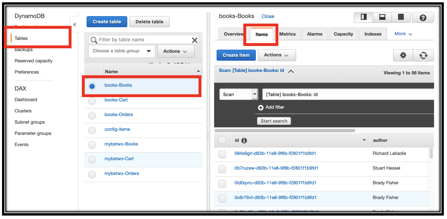
Change the author of a book in DynamoDB

Since you've deployed this application, you deserve a reward! Let's make you the instant author of your favorite book in the bookstore.

Open the DynamoDB console
On the left, select Tables. In the middle, select your -Books table. At the top, select Items
Scroll through the table, looking at the Name column, and pick your favorite.
Hover over the author column, and click the pencil icon to change the Author name to your name. Make sure to click Save to save your changes.

Refresh the bookstore page. Type the title of the book, or your name, in the search bar. Congratulations, you are an author in your own personal bookstore. That was fast - no messing around with publishers, or authoring books! You became an author in seconds.

This example illustrates DynamoDB Streams to Amazon Elasticsearch Service interation. When you make a change in DynamoDB, it emits a record to its stream. You can refer back to the CloudFormation template, and find the table definition by searching for TBooks. Note the StreamSpecification property, which tells DynamoDB to send NEW_AND_OLD_IMAGES to the stream when items change.

The Bookstore Demo App uses a triggered Lambda to catch items in the stream and update the Amazon Elasticsearch Service domain. You can find the definition of the update function in the CloudFormation template. It's named UpdateSearchCluster. Navigate to the Lambda console and type \<project name>-UpdateSearchCluster in the filter. Find and click the Function name to see the Function configuration

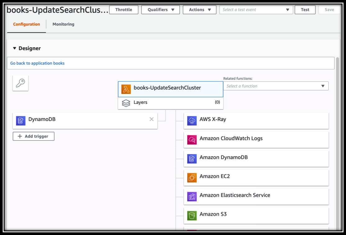
Changes to your source of truth, DynamoDB in this case, propagate out to many of the services using this methodology - DynamoDB Streams triggering a Lambda function to propagate your data across your application.

At the top of the Function configuration section, you can see the triggers for the function on the left (DynamoDB) and the permissions this function has for accessing other services (AWS X-Ray, Amazon CloudWatch Logs, etc.) The permissions are set by the Execution role for the function. Towards the bottom of the page, below the code editor, find the Execution role section. At the bottom, you can click View the \<project name>-ESSearchRole to view the role in the IAM console. You can also find its definition in the CloudFormation template, by searching for ESSearchRole.

Briefly examine the code in the Function code section. The function loops through the event records, and either removes the document from Elasticsearch or updates it depending on the value of eventName.

A final thing to note is that the template sets Environment variables based on the resources it has created. This is how the Lambda function receives the ESEndpoint, for example, without your having to configure it manually. This is a very common pattern - passing resource names, ARNs, endpoints, etc. through environment variables to templated Lambda functions. You can see how these values are wired up by examining the declaration of the UpdateSearchCluster function.

Manually edit the leaderboard/Best Sellers list

First, make sure you have at least two books in your Past orders list with different order quantities.

Scroll down a bit to the Cookbooks section.
Click the Add to cart button for each of these to get 4 books in your cart.
On the Cart page, set the quantity of one of the books to be 1000. You can set the others to different numbers, or leave them at 1.
Click Checkout and then Click Pay.

Don't worry, we won't charge you! You can leave the credit card information as-is, it's not validated. Please don't use your actual credit card information.

You can examine your order by returning to the home screen (click the icon at the top of the page). At the top right of the home page, click Past orders

You can similarly examine the Best sellers.

Unless you've already created multiple accounts for the book store, the books in your Past orders list will match the books in the Best Sellers list (since the bookstore started with no orders).

You ordered 1000 copies of one of the books to bump it to the top of the list. That was clearly an ordering error, so let's go correct the Best Sellers list.

Open the DynamoDB console and find the \<project name>-Orders table.
Find the entry for your big order and click the item to edit it.
Open the "books" list, and then edit the "quantity" to be less than one of your other ordered books. I ordered 3 item of each of 3 books, and 1000 of Scream Ice Cream. I set the order quantity to 2 for Scream Ice Cream.
Click save.
Wait a few moments, and then go to the bookstore endpoint and refresh the Best sellers page. You should notice the book moved in the list.

Just like with updating the search experience, in the backend, DynamoDB Streams automatically pushed this information to ElastiCache for Redis, and the Best Sellers list was updated.

Use AWS X-Ray for call graph and timing

You're a pro at the application architecture. But do you know how long it takes to load your pages? Or, where the time is spent in processing your requests? Or even the dependencies between the different services and Lambda functions? The Bookstore Demo's application architecture is sending all of this information to AWS X-Ray.

AWS X-Ray is a service that collects data about requests that your application serves, and provides tools you can use to view, filter, and gain insights into that data to identify issues and opportunities for optimization.

X-Ray is distributed tracing on the AWS cloud. If you're not familiar with distributed tracing, here are a few key concepts:

Segments the resources in your application send data about their work as segments. A segment provides the resource's name, details about the request, and details about the work done.
Subsegments break down the work of a segment into finer granularity. They include timing information and downstream calls for segments.
Traces A trace ID tracks the path of a request through your application. A trace collects all the segments generated by a single request.

A benefit of building a serverless application is that every AWS Lambda function can send trace data to X-Ray. You can enable this tracing with a simple, "check-box" Boolean.

The Bookstore Demo App comes with X-Ray enabled for all of its API functions and services. While you've been playing with the demo, you've been generating trace data!

Find the FunctionListOrders in the CloudFormation template. Scroll down to the TracingConfig. Setting this to Active is all it takes to generate the X-Ray data you'll examine in a minute.

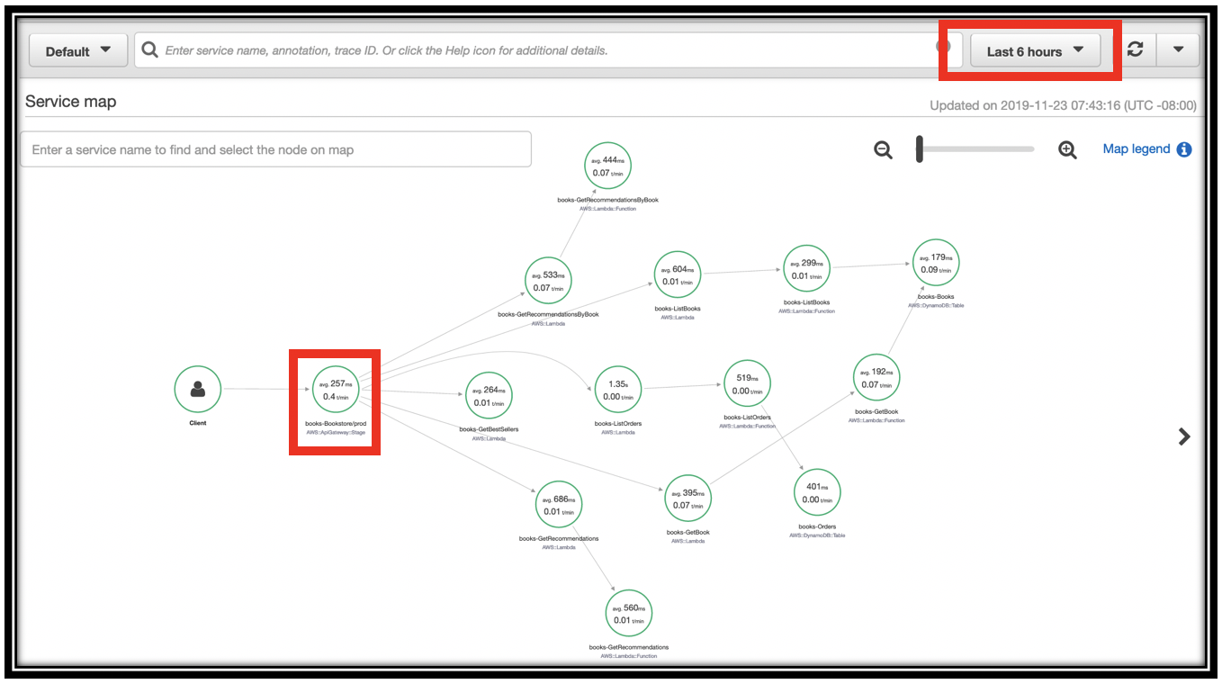
Your Service Graph

X-Ray uses the data that your application sends to generate a service graph. Each AWS resource that sends data to X-Ray appears as a service in the graph. Edges connect the services that work together to serve requests. Edges connect clients to your application, and your application to the downstream services and resources that it uses.

Navigate to the X-Ray console. Make sure Service map is selected in the left navigation pane.
The console initially starts with a 5 minute window. If you don't have data, use the time selector at the top-right of the screen to expand the time.
Zoom in to the leftmost node in the graph (the Client node). Traffic from the client moves to Amazon API Gateway, to the right.
Click the \<project name>-Bookstore/prod node. This reveals aggregate timing information from all of the API calls you've made.
Continue exploring the service graph to see the different calls you made, and the services they invoked. Direct children of the API Gateway node are the Lambda functions backing your API. I have \<project name>-GetBestSellers, \<project name>-GetBook, \<project name>-ListOrders and many more.
You can see throughput, timing, and error information at each level of the tree. For instance, \<project name>-ListOrders calls AWS Lambda for the \<project name>-ListOrders function. AWS Lambda then invokes the \<project name>-ListOrders function (next node). The function calls Amazon DynamoDB (leaf node)
Click one of these nodes to see details on the timing

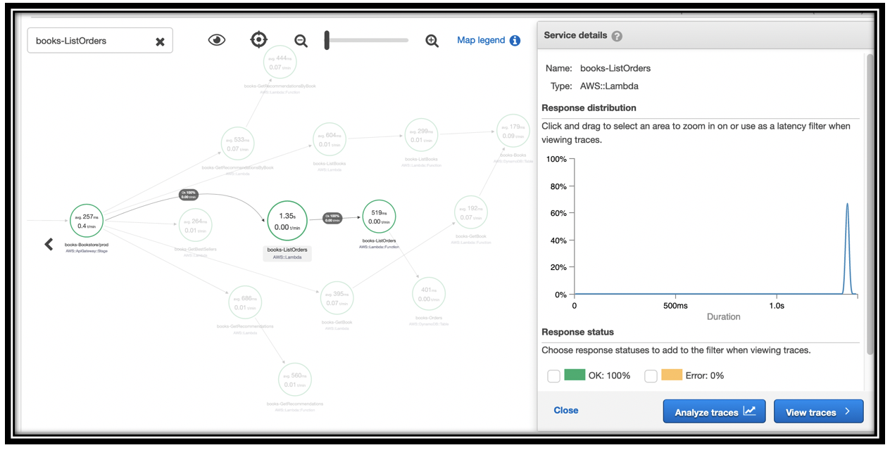
In my case, I only called ListOrders once, taking 1.35s. You can see that the downstream function call time is 519ms.

Continue to explore the service map to get a visual feel for how the Bookstore Demo App is constructed, the dependencies, and timing and latency.

Explore traces

The segment map is a way to visualize an overview of your API request processing. To get deeper information, you explore traces.

Navigate to the Bookstore home page.
Type Lamb in the search bar and press enter. You receive one search result
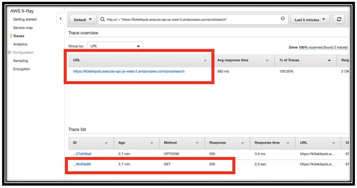
Navigate to the X-Ray console
Select Traces from the left navigation pane.
Set the time selector to Last 5 minutes.
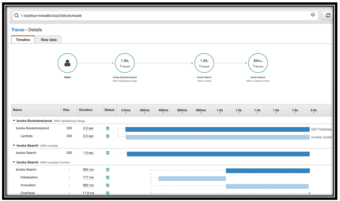
Locate and click https://\<application endpoint>.execute-api.us-west-2.amazonaws.com/prod/search in the URL section of the page.
You will have 2 traces one for the OPTIONS method and one for the GET method. Click the ID for the trace of the GET method.
Look at the details for this trace. At the top, you can see the call graph for just this function. The \<project name>-Bookstore/prod time is completely covered by the call to Lambda.
The \<project name>-Search Lambda function details show the Initialization time, the Invocation time, and a small amount of overhead. In my case, Initialization took almost as long as Invocation.
Return to the Bookstore home page and search for Cookbooks.
Return to the Traces tab, and find this second request. You can see that the time has reduced considerably (in my case, 700ms, down from 2.5s). The Lambda function is warm.

Troubleshoot a slow function

Let's simulate a problem with the Bookstore's \-Search function.

Navigate to the AWS Lambda console.
Type \<project name>-Search in the search bar (*be sure to replace \<project name> with your project's name.
Click the URL for your function.
To simulate a problem, add the following code, right after the start = int(time.time()) statement

if event["queryStringParameters"]["q"] == "Cookbooks": time.sleep(5)
Click Save to save the function.
This simulates a condition where a particular query runs slowly.
Return to the Bookstore home page. and search for Lamb, Databases, Floor, and Cookbooks (a few times)
Note: you must return to the bookstore home page before each search. The search results page is not correctly configured to execute searches.
Navigate to the X-Ray console.
Select the Analytics tab in the left navigation pane.
Set the time selector to Last 5 minutes (or a time period covering the searching you just did).
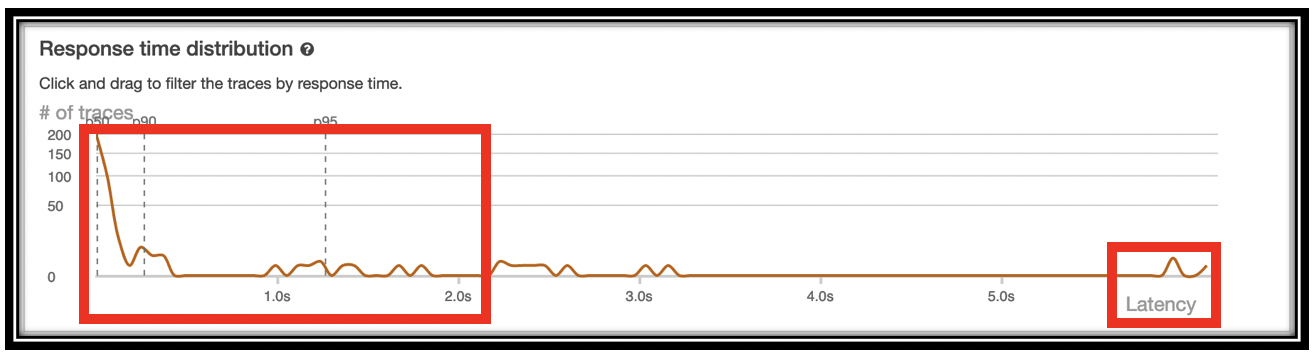
You can see a bimodal distribution of response times.
Click and drag on the timeline for the high latency requests to filter to that latency window
Examine the Time series activity panel to see when these requests occurred and how they compare with the other requests, both concurrent and historically.
Scroll down further to the Trace list pane.
You can see your requests, with latencies all higher than 5 seconds. These are all invocations of the search function. In normal debugging, you would go to the Search function, instrument it further and/or explore Amazon Elasticsearch Service logs to fix the problem.
Select one of the traces to view the Trace details page.
Click the Raw data tab.
Review the data and structure of the trace, its segments, and its subsegments.

That's an excellent segue to the next section, where you'll dig deep into the performance of your application with Amazon ES.

You've barely scratched the surface of distributed tracing. While the information provided is very useful, the automatic instrumentation is shallow. Where it gets really interesting is when you add your own tracing information via the X-Ray SDK.

Troubleshoot an error

When you deploy the Bookstore, CloudFormation can complete before Neptune has fully stabilized. In that case, you might see "Network error" dialogs. If this is already happening... don't worry! It will stop once Neptune is fully available. You can troubleshoot this problem with X-Ray.

If this is not happening to you... don't worry! You'll simulate that issue now.

Navigate to the Lambda console.
Type books-GetRecommendations in the Functions text box.
Click books-GetRecommendations.
Scroll down to the code editor and locate the response = {... specification.
Just before that, add the following code:

raise Exception("Oops")
Save the function.
Return to the Bookstore home page, and reload the page. You will receive an error dialog.
Reload the page several more times.
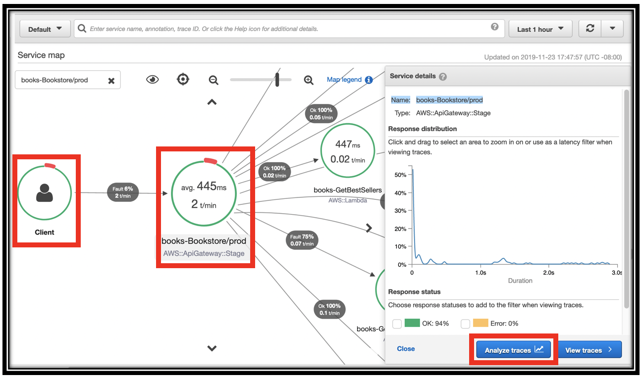
Go to the X-Ray console, Service map.
You should see that the green circle around the Client now has a small red bar.
Click the \<project name>-Bookstore/prod node in the graph.
Click Analyze traces.
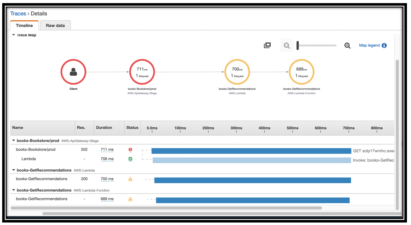
Scroll down to the HTTP STATUS CODE section.
Click the row for status code 502.
Scroll to Trace list at the bottom of the page. By inspection, you can see that the problem is with the recommendations API.
Click one of the traces to see the details. You can see that the call to \<project name>-GetRecommendations has a status code of 502, and the Lambda duration is pending.
You can click the yellow triangle to see the raw details of the error.
Before continuing to the next section, remove the Exception from the GetRecommendations function and save it.

Explore Amazon Elasticsearch Service and Kibana

You know a ton about your application, its infrastructure, and the tracing of requests with X-Ray. Now it's time to dig in a little deeper and augment trace information with logging and metric information that the Bookstore demo stores in Amazon ES.

Amazon Elasticsearch Service is a fully managed service that makes it easy for you to deploy, secure, and operate Elasticsearch at scale with zero down time. The service offers open-source Elasticsearch APIs, managed Kibana, and integrations with Logstash and other AWS Services, enabling you to ingest data securely from any source and search, analyze, and visualize it in real time.

Here are some of the key concepts for Amazon Elasticsearch Service.

Domain: Elasticsearch is a distributed database that runs in a cluster of nodes. Amazon Elasticsearch Service domains comprise a managed, Elasticsearch cluster, along with additional software and infrastructure to provide you with API access to Elasticsearch, and access to Kibana (a web client that we'll explore in depth).
Index: Data in Elasticsearch is stored in indexes. You can think of an index as being akin to a table in a relational database. When you index data, or send queries, you specify the target index as part of the API call.
Shard: Each index comprises a set of shards - primary or replica. Each shard is an instance of Apache Lucene, which manages storage and processing for a subset of the documents in the index. Shards partition the data in the index so that Elasticsearch can distribute storage and processing across the nodes in the cluster.
Index pattern: When you use Amazon ES for logging and analytics, you use an index per day (usually) to store your data. That way, you can DELETE old indexes for lifecycle management. Your index names contain a root string like "appdata", along with a timestamp. When you use Kibana, you use the root string with a wildcard to specify the set of indexes - the index pattern.
Document: A document, for logging, is a single log line, as a JSON object. More generally, a document is the main entity that you index and that you retrieve with queries. A document is like a row in a relational database.
Field: A field is a single key from a JSON document. It's like a column in a relational database.

In this part of the lab, you will build a Kibana dashboard to monitor your application.

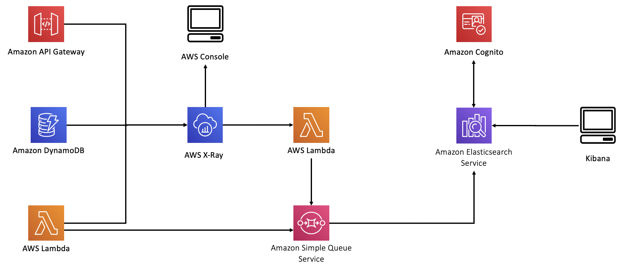
Explore the ingest architecture

The Bookstore Demo uses an Amazon Simple Queue Service (SQS) queue to forward trace information from X-Ray and logging information from the functions backing the API to Amazon Elasticsearch service.

The Bookstore Demo is deployed in an Amazon Virtual Private Cloud (VPC). To enhance security, the VPC does not have an Internet Gateway or a NAT Gateway to allow traffic in or out of the VPC. For demo purposes, we chose to host the logging infrastructure outside of the VPC to make it easy to access Amazon ES and Kibana.

In a production deployment, the logging infrastructure should all reside within a VPC. Provide access to Kibana with a tightly-secured NAT gateway and a proxy for the Amazon ES domain.

Open the CloudFormation template.

You can find the queue definition by searching for LoggingQueue.
Follwing the LoggingQueue, you will find a VPC endpoint definition along with a security group. This allows the Lambda functions to communicate with SQS from within the VPC.
Further down, you can find the XRayPullerFunction this function calls X-Ray's API, parses and forwards the trace and segment information to SQS. The template also defines a scheduled event to run the X-Ray puller every minute.
The SQSPullerLambda, which runs outside of the VPC, retrieves items from the queue and forwards them to Amazon ES.
The AnalyticsElasticsearchDomain defines the endpoint for log shipping. It's also hosted outside the VPC

Set up Kibana

The Bookstore Demo uses Amazon Cognito to provide authentication and access control for the logging domain. For the purposes of the demo, we used the same User and Identity pools that support login for the app. Of course, in a real deployment, you'll use a separate User and Identity pool to provide access for your own staff (as opposed to your end users!). Using the same pool has the advantage that you can log in to Kibana with the same credentials you used to log in to the app.

Navigate to the Amazon Elasticsearch Service console.
Find and click the \<project name>-logs domain in the left navigation pane.
Click the Kibana URL.
In the sign in dialog, enter the Email and Password for the account you created in the Bookstore app.
You'll see a welcome screen. Click Explore on my own

In order to work with the data in Amazon ES, you need to tell Kibana the index patterns for that data. Kibana retrieves the mapping for each of these index patterns. It uses the mapping when deciding, for example, whether you can sum the values in a particular field (are they numbers?). Your first step in Kbana is to create these index patterns. You do this on the settings tab.

Click the icon in the left navigation pane to navigate to the settings pane.
Click Index Patterns.
In the Index pattern field, type segments-* and click Next step
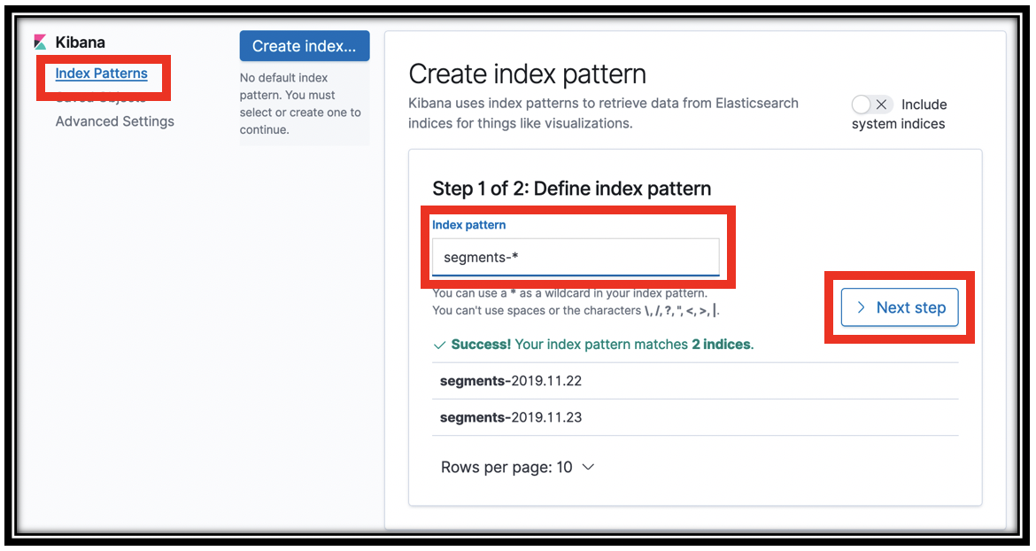
In step 2 of the wizard, choose \@timestamp from the Time Filter field name menu.
Click Create index pattern. Kibana queries Amazon ES to find the schema for these indexes and shows that schema to you.
Repeat the process by clicking the Create index pattern button to define an index pattern for summaries-* and appdata-*.

You've now set up Kibana with your indexes and their mappings to be able to create visualizations.

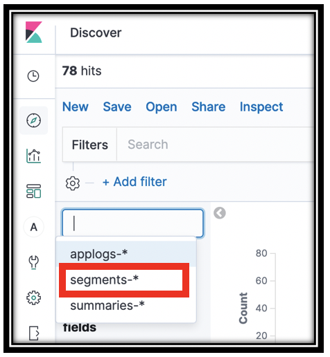
Use the Discover pane

The Discover pane provides an overview of the index pattern you select. It's a quick-start location, where you first go to see that there is data in your index, search across that data, and see the fields and values of your documents.

Click the in the left navigation pane to navigate to Kibana's Discover panel.
Make sure that you are looking at the segments-* index pattern. At the top left, drop down the index patterns menu, and select segments-*
Depending on the time elapsed from when you last worked with the Bookstore app, you might receive No results match your search criteria.
Drop down the time selector menu, which shows as a calendar icon at the top right of the screen. In the Commonly used section, click Today. The time selector keys off of the \@timestamp field of the index pattern.
You now have a histogram with the event counts for events that were logged to the segments-* index at the top of the screen.
Below that are sample records in the index. Use the disclosure triangle to open one of the segment records. When I did that, I found a Mock record. Well, that's not what I want! Let's employ Elasticsearch's search function to narrow to relevant records!
In the Filters search box, type trace_type:segment to narrow the displayed documents to only segments. (The trace_type field was added by the XRayPuller function to help route data into different Elasticsearch indexes. If you're curious, you can have a look at the trace_details_sink.py file in that function)
Open the disclosure triangle next to one of the records. You may be looking at a root segemnt, or one of the subsegments. trace_details_sink flattens the trace structure that X-Ray generates, producing a single record at each level of the tree. Examine the fields and values for some of the records to get a feel for this data

Kibana can also show you a tabular view of your data. This is a powerful way to dig in and narrow to the interesting records. You can use this to find log lines that surface information about infrastructure problems. For example, you can quickly build a table of requests and result codes.
Hover over one of the field descriptions in an open document to reveal the icons on the left. Click the table icon to put that value in a table.
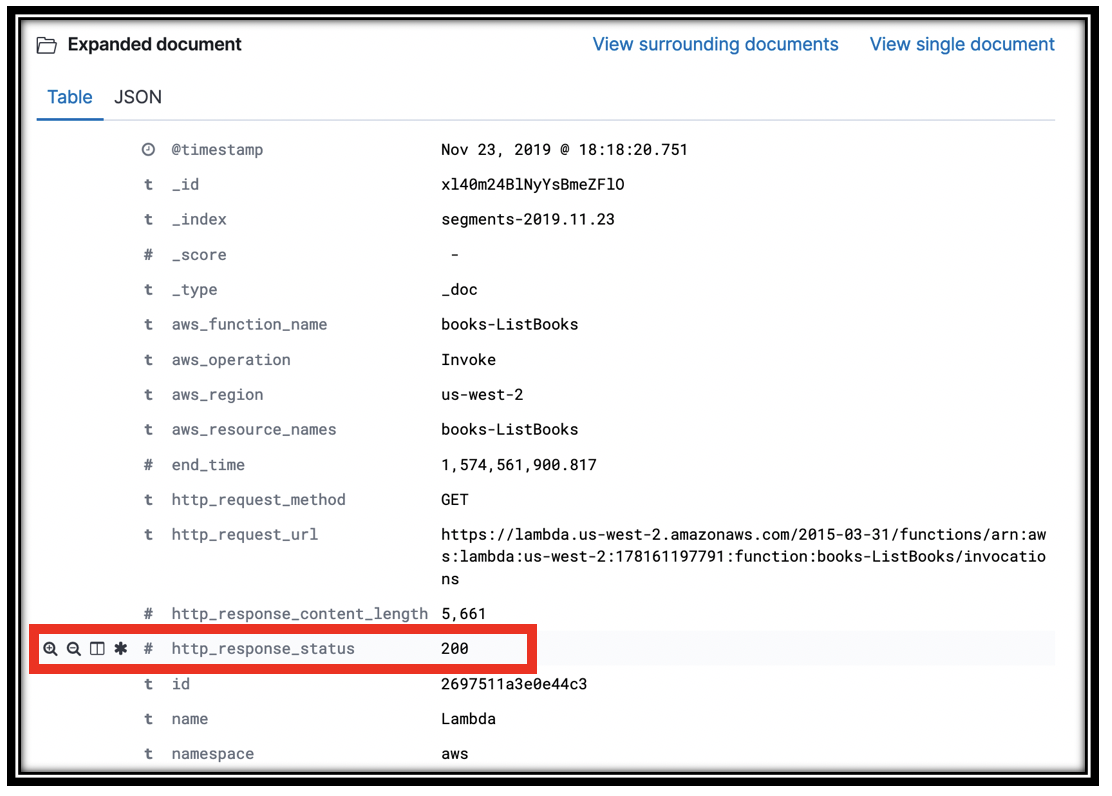
Add the Trace ID, http_response_code, aws_operation, aws_function_name, and any other fields that look interesting.
Scroll up to find the discover triangle and close it. You are now looking at a table with the rows you selected.
Find a row with 200 in the http_response_code. Hover over the value, to reveal 2 magnifying glasses, one with a plus sign and one with a minus. These are quick links that let you Filter for or Filter out a value. Click the magnifying glass with a minus sign to filter out segments with a 200 response.
You can remove this filter later at the top of the screen, right below the search bar.
Find a row with a 502 and Filter for that value to reveal the segments from the failed GetRecommendations calls you simulated above.

Visualize your data with Kibana

You've seen that Kibana provides you with an intuitive search front end for the data in your logs. You can also build visualizations that provide you with monitoring of your underlying infrastructure and application.

The Bookstore app sends data from X-Ray and the Lambda functions themselves. You have set up index patterns for trace segments, and application logs. Let's pull some information out of that raw data.

A simple visualization: call duration

Calls to the Bookstore app come through the API Gateway and are rendered as traces in X-Ray. You can find this data in the trace summaries-* index. The summary data does not have a timestamp, but you can still do some interesting analysis. Let's visualize the aggregate Duration for each of the Lambda functions.

In the Kibana left navigation pane, click the icon.
Click Create a visualization
In the New visualization dialog, scroll down and click Vertical bar
In the New Vertical Bar/Choose a source dialog, click the summaries-* index pattern.
The visualization panel opens. In this pane you choose the fields to graph on the X- and Y-axes.
In the Metrics section, click the disclosure triangle and select Average from the Y-Axis menu
From the Field menu, select Duration
Under Buckets select X-Axis
Drop the Aggregation menu and select Terms (you might have to scroll the menu to see it)
In the Field menu, choose function_name.keyword
Click the Update icon .

You created a histogram showing you the average Duration for the invocations to your Lambda functions.

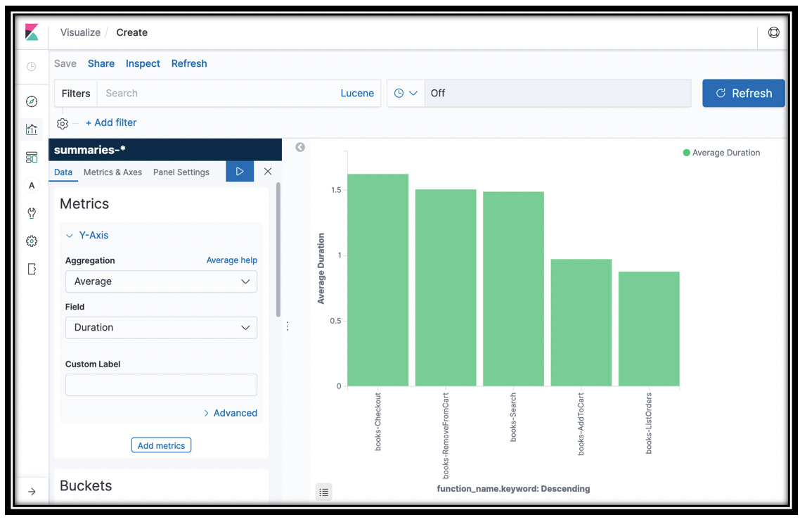
Bar chart showing average call duration

We'll use this visualization in a dashboard in a bit. 1. Click Save at the top left of the window. 2. Name your visualization Average lambda duration and click Confirm save

[Optional]: You can add sub-buckets to get a stacked bar chart. Try adding a sub bucket with a Terms aggregation on the ResponseTimeRootCauses.Services.Name.keyword. Or, build a Vertical Bar visualization from the segments index (by selecting the segments-* index pattern when creating the visualization), with a vertical bar for aws_function_name.keyword, with http_response_code (scroll down to the number section of the Field menu) sub aggregation.

Examine the application data

The previous visualization shows some of the power of Kibana. Kibana really shines when working with time-based data like the trace segments and application data. You're going to build several visualizations for application data and collect those as a dashboard. First you need to understand what's in that data.

You could use the discover pane for this. Kibana has another pane, the Dev Tools pane where you can send Elasticsearch API commands directly to Amazon ES. This is more free-form, but lets you peek under the covers in more depth.

Click the icon to go to the developer tools tab
If this is your first time opening this tab, click Get To Work
To see all of the indices type GET _cat/indices?v and then click the update icon . You may notice that Kibana helpfully offers you auto-complete suggestions as you type.

You should see 5 indexes: - applogs-YYYY-MM-DD: holds data from searches, addToCart and Checkout - summaries-YYYY-MM-DD: holds data from X-Ray's summaries APIs - segments-YYYY-MM-DD: holds data from X-Ray's segments APIs - .kibana1: This is Kibana's own data. When you set up index patterns, create visualizations, and create dashboards, Kibana saves the configuration information here. - \<project name>-timer*: we used Amazon ES to store a timestamp for the X-Ray puller function. This index contains a single document with the last time data was retrieved from X-Ray
To search an index, you use the _search API. Type or copy the following search request to see all of the data in the applogs-* index.

GET applogs-*/_search { "query": { "match_all": {}} } The match_all query, as implied, matches every document in the index. When you have entered the above, click the icon to see the results. 5. You are looking at a mix of data. You can see that all of the records have a trace_type of appdata. All records also have an appdata_type
- search_result: each search result is logged, including client_time, query keywords, and a hits_count (the total number of results for the query)
- hit: Each hit (search result) is also logged. The data is taken from DynamoDB and flattened. You can see the book's category (Category_S), its name (name_s), author (author_S), price (price_N), rating (rating_N), and more.
- purchase: The Checkout Lambda logs each purchase, including each book's name (book_name), category (book_category), author (book_author), price (book_price), total_purchase amount (total_purchase) and more
- add_to_cart: The addToCart Lambda logs each time a book is added to the cart (not the same as purchased!). You can see the book's name (book_name), category (book_category), author (book_author), price (book_price), and more
- You may not have seen each of these types of record. You can search for a particular record set (and you'll use it to narrow your visualizations later) by searching for the appdata_type. Enter the following:
GET applogs-*/_search { "query": { "term": { "appdata_type": { "value": "hit" } } } }

Use Kibana's update icon to run the query. The term search looks for a match in a text field. 7. Kibana's aggregations provide analysis of the data in your fields. Continuing with the search hits, you can see the distribution of categories for the books surfaced. Enter the following:

GET applogs-*/_search { "query": { "term": { "appdata_type": { "value": "hit" } } }, "aggs": { "Categories": { "terms": { "field": "category_S.keyword", "size": 10 } } }, "size": 0 }

Run this query by clicking Kibana's update icon. You added an aggs section to the query to have Elasticsearch build buckets for each of the category_S.keyword values. You can see how many hits documents were in each category in the result.
You also set the size to 0. The from and size query parameters enable you to do result pagination. You set size to 0 because you didn't want to see search results, just the aggregations.
[Sidebar: To support free-text searches, you use text type fields. For exact matches you use keyword type fields. When Elasticsearch first sees your data, it infers a type for each field. For maximum flexibility, when it sees text data, it creates a field (FIELD) for free text matching and a duplicate, sub-field (FIELD.keyword) for keyword matching. The category_S.keyword field is the keyword copy of the text data in the category_S field. The reasons for this are complex, but you'll get a hint if you forget to add the .keyword to the field name in the aggregation above. By default, Elasticsearch stores columnar data to support aggregations for keyword fields but not for text fields.]

Kibana uses the aggregations APIs to collect data to display in visual form. You just built a category histogram for the categories of books that were returned in search results. You could have done the same if you had instead built a Vertical Bar visualization in Kibana. Kibana would build bars, X- and Y-Axes, according to the buckets and values you retrieved.

When you build search applications, you use the same kinds of aggregations to surface buckets that your customers can use to narrow search results. You display the bucket names and counts in your left navigation pane, and when customers click the bucket, you add that value to the query to narrow the results.

Optional: You can simulate this behavior by running the following query:

GET applogs-*/_search
{
  "query": {
    "bool": {
      "must": [
        {"term": {
          "appdata_type": {
            "value": "hit"
          }
        }},
        {
          "term": {
            "category_S.keyword": {
              "value": "Database"
            }
          }
        }
      ]
    }
  }
}

The bool query provides the means to mix multiple clauses. In this query must clauses must all match for the document to match. In other words, this query retrieves documents (log lines) whose appdata_type is hit AND whose category_S.keyword is Database.

Build a timeline visualization

You can use Kibana's time series visualization to see an overview of how customers are interacting with your application.

First, spend some time in the Bookstore front end. Run some searches, add some items to the cart, and make multiple purchases.

(Note: there's a bug in the UI, you can't search again from the search results page. Instead, click the icon to return to the home page)
Click the visualization icon (). If you are looking at a previous visualization, click the visualization icon again. Two clicks clears a current visualization.
Click the Plus icon to create a new visualization
Scroll down and click Visual Builder
In the visual builder, select Terms from the Group By menu.
Select appdata_type.keyword from the By menu.
Click Save (top left) to save your visualization as KPI Time Series

The resulting visualization shows you a count of search_result documents (log lines), add_to_cart documents, purchase documents, and hits documents. This high level view tells you how your customers are interacting with your catalog.

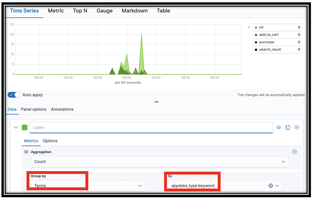
Kibana visual builder showing key performance indicators

[Optional] You can also filter the documents to remove, e.g. the hits from the graph. Select the Options tab in visual builder. In the Filter box, enter NOT appdata_type:hit. The chart updates to remove hits.

[Optional] Experiment with building time series visualizations for other fields. There is rich data in the segments-* index. Set the index pattern in the Panel options tab. Try visualizing aws_operation.keyword or http_response_status in the Data panel Group By selectors for example.

What are your customers searching for?

The Search function is logging the keywords from your customer queries. You can visualize these keywords with a vertical bar, or you can use a tag cloud to see them.

Click the visualization icon, twice if you need to
Click the Plus icon
Select the applogs-* index pattern
In the Buckets section, click Tags
In the Aggregation menu, select Terms
In the Field menu, select query.keyword
Click the update icon to see a tag cloud of your customer queries
Save the visualization as Query cloud

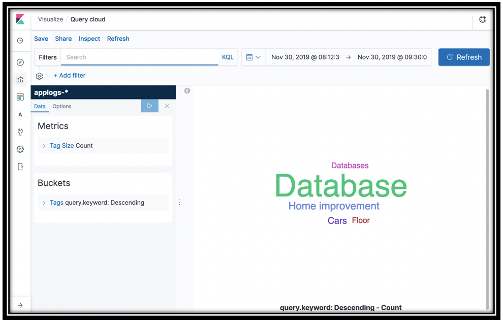
Kibana tag cloud visualization with search query words

[Optional] What's even more interesting is to see what's missing from your catalog. In the Filters box, type hits_count:0. You might have to go back to the Bookstore Demo and search for something crazy like asdf to have data if you don't already have some empty search results. This information can guide you on building out your eCommerce catalog, or figuring out which features are not working properly for your customers.

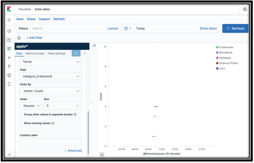
Work with line graphs

You use line graphs for tighter control over how you monitor values for your application's KPIs. You graph the sum, average, max, or min of a numeric field on the Y-Axis and use the X-Axis to bucket by time. You narrow or expand the time window to control the data in the graph.

In Kibana, click the visualization icon, twice if you need to
Click the Plus icon on the top-right
Click Line
Choose applogs-* under Choose a source

When you work with time series data, first you set a date histogram for the X Axis, then you choose a numeric aggregation like Sum or Max of a field for the Y axis. To further decompose your data, you add sub buckets on the X axis.

Under Buckets, Click X-Axis
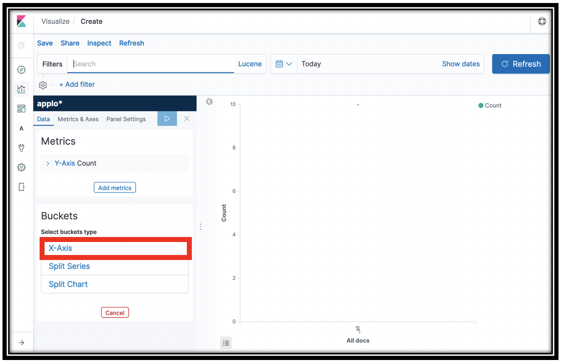
In the Aggregations menu, click Date Histogram
Click the icon
You now have a count of the items in the applogs-* indexes on the Y-Axis.
Click the disclosure triangle next to Y-Axis
In the Aggregation menu, click Sum
In the Field menu, select the total_purchase field
This line graph gives you the total purchases across time, as captured by the \<project name>-Checkout function. You can examine the log_sale method in the Lambda function to see the records it sends to Amazon ES.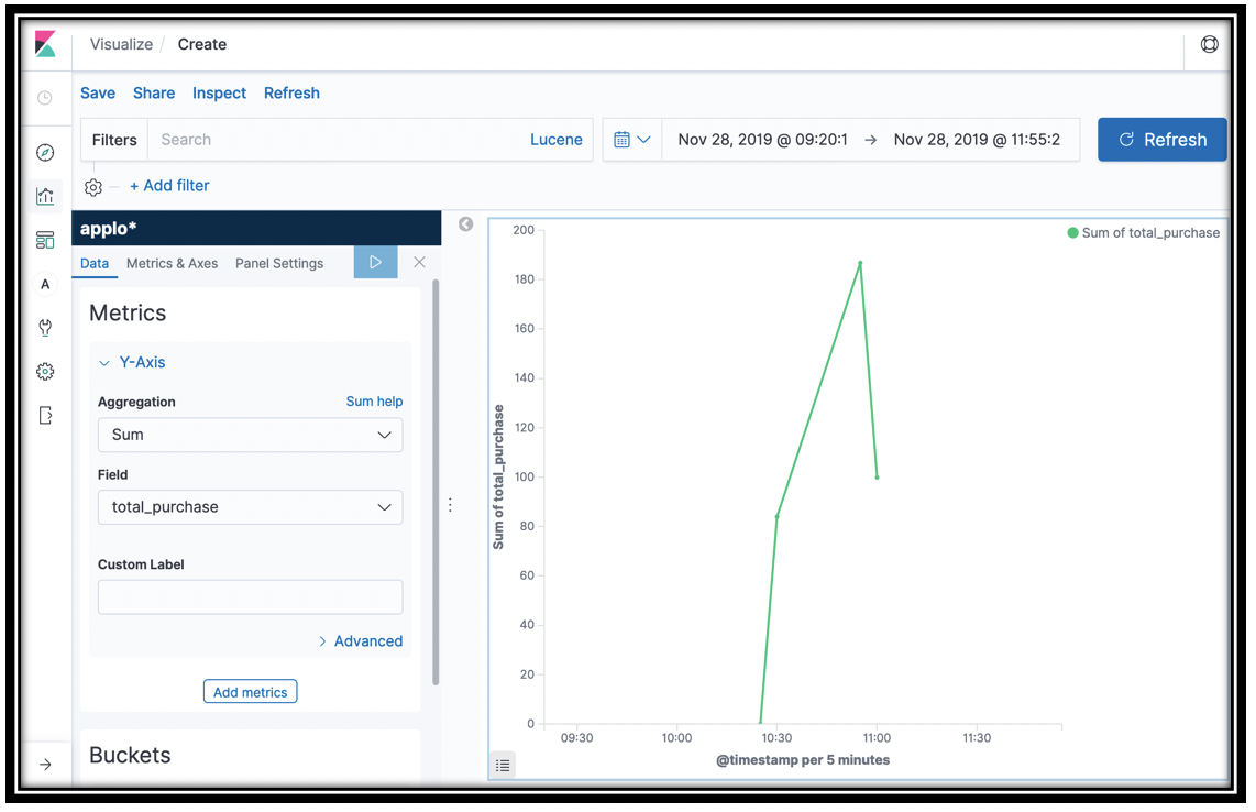
This is not actually quite right. Both addToCart and Checkout record a total_purchase field. Your visualization gathers data from both of these appdata_types, since they're in the same index. In order to see purchases from Checkout only, you need to add a Filter. In the Filter box, type appdata_type:purchase.
[Optional] Another alternative is to graph both add_to_cart and purchase using a Terms sub aggregation on the appdata_type field. Or you can use a Filters sub aggregation to select add_to_cart or purchase explicitly

You might wonder why we added a total purchase to the addToCart function. By viewing both adds and purchases, you can see what orders your customers are abandoning in their carts. You can further dig in to try to diagnose the cause to increase revenue.

Click Save and save the visualization as total sales
Let's continue with this graph to find out purchases by category
Scroll down and click Add sub-buckets under the Buckets portion of the left navigation pane.
Click Split Series under Select bucket type
In the Sub aggregation menu, scroll down and click Terms
In the Field menu, scroll down and click book_category.keyword
Click the update icon
Click Save
Click the slider to Save as a new visualization
Name the visualization sales by category
Click Confirm Save

These two line graphs show you total purchases over time, and purchases by category over time.

[Optional] What other line graphs can you build? The segments-* index contains deep data about the calls for the back end. For example, you can graph the http_response_status by aws_api_gateway_rest_api_id. You can add a filter to limit the graph to a particular aws_operation. Or you can build a line graph of aws_operation. Want to see DynamoDB only? Add a Filter name:DynamoDB. Use GET segments-*/_search in the Dev Tools panel to dig in to the fields available and get creative!

Understand your customers' search behavior

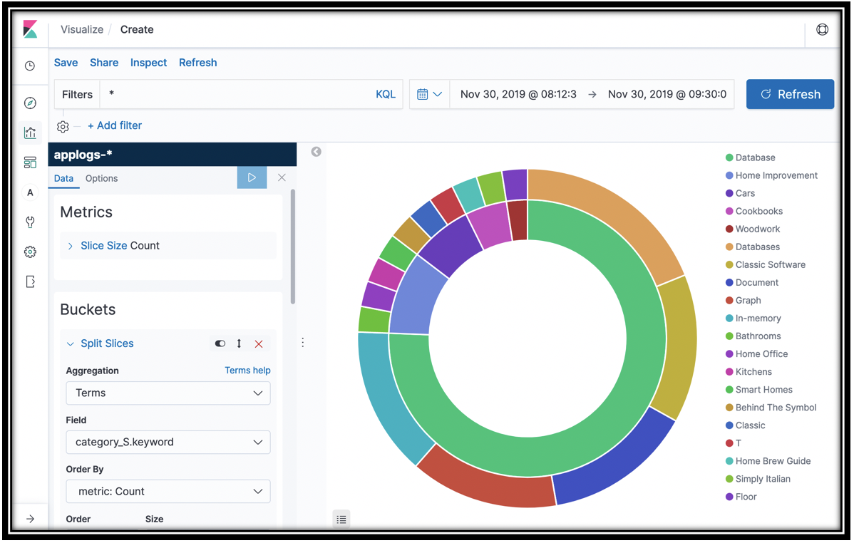
Let's see which caegories and products are most often retrieved by customer searches. You can do this with a pie chart.

Click the visualization icon in Kibana's left navigation pane
Click the "plus" icon at the top-right of the screen
Click the Pie icon
For Index pattern, click applogs-*
Click Split Slices
Select Terms from the Aggregation menu
Select category_S.keyword
Click the update icon
You have the top 5 categories that appeared in search results. To subdivide, scroll down in the left navigation pane, and click Add sub-buckets
Click Split Slices under Select buckets type
Select Terms from the Sub Aggregation menu and name_S.keyword from the Field menu.
Save your visualization as Search result books

You have the top 5 categories and the top 5 books in each category that customers saw in search results. You can find the source of this data in the \<project name>-Search Lambda function.

[Optional] Explore the segment and summary data as well. From the summary data, chart out the function_names.keyword and sub-bucket by ResponseTimeRootCauses.Services.AccountId.keyword (second menu choice) to see which accounts (customers) are using which functions.

Build your dashboard

The visualizations that you've built are great for ad-hoc, root-cause diagnosis and repair. For ongoing monitoring, you collect your visualizations in a dashboard that you can monitor in real time.

Click the icon
Click Create new dashboard
Click Add either in the revealed dialog, or at the top-left of the screen.
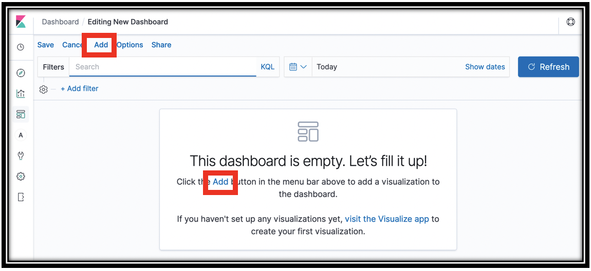
From the Add Panels slide-out drawer, click visualizations to add them
Close the drawer
You can move by dragging, and resize the visualizations
When you're done, click Save and name your dashboard KPIs
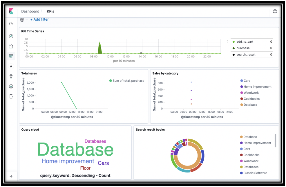
To update your dashboard in near real time, drop down the time menu (top-center of the screen). You use this menu to control the time frame for dashboards and visualizations across Kibana.
Under Refresh every, type 10 in the text box and click Start
Your dashboard will now refresh every 10 seconds with new data. Run some more searches, cart adds, and checkouts to see this.

[Optional] Set an alert

You have created a dashboard so that you can monitor what's happening in your application in real time. In reality, you want automated monitoring with alerting based on the contents of your log data.

Amazon Elasticsearch Service Alerting is a powerful framework for setting alerts on your application data. You build a Monitor query to pull a value from your logs. You set a Trigger threshold with one or more Actions to deliver a message to a Destination like Slack, Amazon Chime, or even a custom webhook.

Follow the instructions here to set up alerting in Amazon Elasticsearch Service for your \<project name>-logs, Amazon ES domain.

Add an alert for http_response_code >= 300 and get notified when your application is having issues. Or, add an alert for aggregate total_purchase < some value to get notified of a sales drop.

Cleanup!

To make sure you don't continue to incur charges on your AWS account, make sure to tear down your applications and remove all resources associated with both AWS Full-Stack Template and AWS Bookstore Demo App.

Log into the Amazon S3 Console and delete the buckets created for this workshop.
There should be two buckets created for AWS Full-Stack Template and two buckets created for AWS Bookstore Demo App. The buckets will be titled "X" and "X-pipeline", where "X" is the name you specified in the CloudFormation wizard under the AssetsBucketName parameter.
Note: Please be very careful to only delete the buckets associated with this workshop that you are absolutely sure you want to delete.
Log into the AWS CloudFormation Console and find the stack you created during this workshop
Delete the stack

Remember to shut down/remove all related resources once you are finished to avoid ongoing charges to your AWS account.

Build on!

Now that you are an expert in creating full-stack applications in just a few clicks, go build something awesome! Let us know what you come up with. We encourage developer participation via contributions and suggested additions to both AWS Full-Stack Template and AWS Bookstore Demo App. Of course you are welcome to create your own version!

Please see the contributing guidelines for more information.

Questions and contact

For questions on the AWS Full-Stack Template, or to contact the team, please leave a comment on GitHub.